Clinical data from CPTAC-3 are now being made available through an API hosted by ESAC. This is documented in detail at https://clinicalapi-cptac.esacinc.com/api/tcia/.
Loading JSON files into Excel
The following guide has been prepared for researchers who are not used to working with JSON data or APIs. By following these steps you will be able to view the data in newer versions of Excel via the Power Query feature.
To generate the JSON file:
- First access the CPTAC Clinical Data API: https://clinicalapi-cptac.esacinc.com/api/tcia/
- Select “Get clinical data by Tumor Code” from the left navigation Panel

- From the “tumor_code” drop down menu, select the desired tumor type. Click on “Try” to generate the JSON code

- Select and copy the URL from the “Request URL” box. Click 3 times on the URL to highlight the entire string; then immediately right click and select copy)

- Paste the URL into a new browser.
- Click on the 3 vertical dots in the upper right corner of the browser; select “More tools”, then “Save page as”
- Save as a JSON in your file directory.

To Load the Clinical Data file into an Excel Sheet
- Open a blank excel sheet
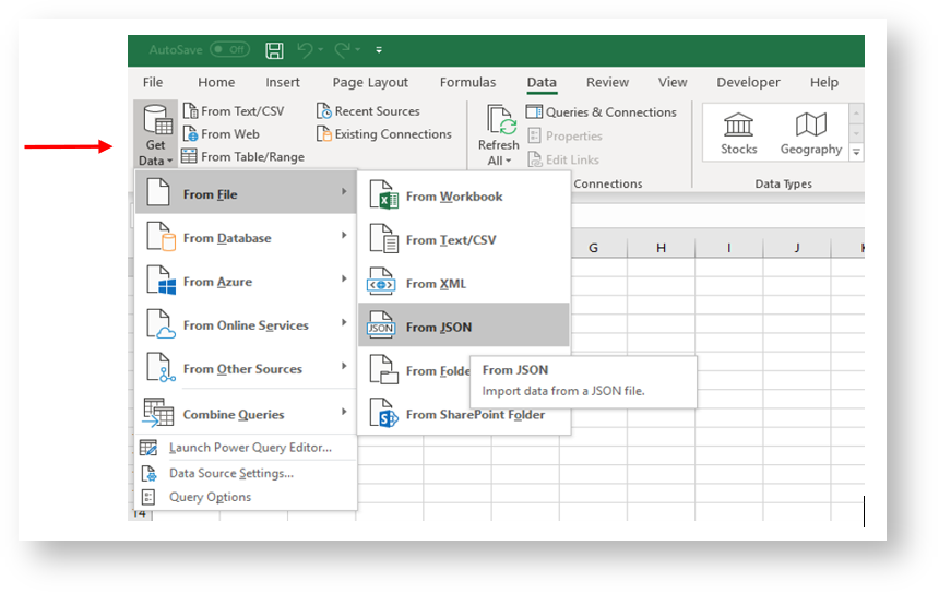
- From the main menu, select “Data”
- From the “Get Data” drop down menu, select “From File”, then “From JSON”
- Select the saved JSON file from your directory.
- From the power query editor select “To Table” from the main menu, to convert the data into a table format.
- In the table window, keep the delimiter and extra column selections as shown below and click on “ok.”

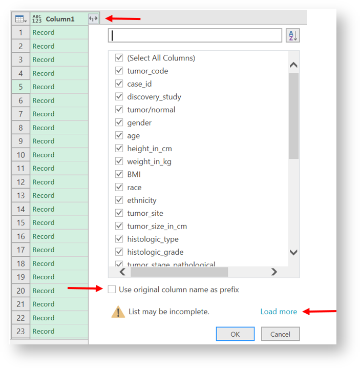
- Click on the expansion arrow icon next to the “Column1” header, then click on “load more” at the bottom of the column header list to ensure all columns are selected.
- Uncheck the box next to “Use original column name as prefix”
- Click on “ok” after the full list has loaded and “ok” again to load all columns into the table.
- The “specimens” column has a sub-level with specimen-related column headings (specimen id, slide id, etc.). To expand the specimens column, use the scroll bar at the bottom of the table and scroll right until you get to the “specimens” column.
- Click on the expansion arrow icon to pull these columns into your table. Then select “Expand to new rows”

- You will notice that the column entries have changed from “list” to “record”. Click on the expansion arrow icon again to open the specimen column list.
- Click on “load more” to ensure all column headings from the specimens table are included, then “ok.” Notice that the number of columns and rows in your table shown at the bottom of the table have now increased.
- Please note that the entries in some columns are now duplicated – for instance for case C3L-00004, the gender and age columns are listed 3 times. This is a result of corresponding specimen IDs and slide IDs for this case being pulled into the table.
Quick Formatting Tips:
- To rearrange columns: click and highlight the column then drag to desired location.
- To select specific column headers: select “choose columns” from the home menu, then select only the column headers you would like to see. The remaining columns will be deleted.
- To remove columns: highlight the specific column and click on “remove column” from the home menu; or select “remove columns” to select multiple columns to remove.
- To remove the “Column1” text in all column headings, wait until you have loaded the table into your Excel spreadsheet.
Changing Format from Table to Excel worksheet
- After you have customized the table, select “Close and Load”
- To save the data as a spreadsheet:
- Highlight the entire worksheet by selecting the triangle icon in the upper left corner of the worksheet
- Right-click anywhere in the table and select copy

- Create a new sheet using the plus sign icon at the bottom of the worksheet
- Click on the triangle icon in the new sheet (or in cell A1); right click and select “paste values”
- Format as desired: make column headings bold; or add column filters by selecting the entire worksheet) and selecting “filter” from the sort and filter menu.
- Delete other worksheets and save your spreadsheet as an excel file.